A classifier that scored 100% and knew nothing
Trained on one acoustic environment, a solid-versus-hollow sphere classifier was perfect. Moved to a second environment, it fell to chance. This note reports the result, the diagnosis, and why we called it a no-go.
- Question
- Does a structural-acoustic target classifier survive a change of environment?
- Data
- Blanford (2024) in-air synthetic aperture sonar, CC BY 4.0: real measured echoes, not simulation
- Targets
- Solid sphere vs hollow sphere (specular return vs elastic resonance)
- Design
- Train on one environment, test on two unseen ones
- Scale
- 60 runs · 2,400 target looks · 50-dimensional features
- Result
- 100% in-environment → 53% out-of-environment (chance = 50%)
- Verdict
- No-go for these features
Why solid versus hollow
A solid object returns sound in essentially one way: the geometry reflects it. A hollow, elastic shell does something extra: it rings. Energy enters the shell wall, circumnavigates it, and re-radiates with a delay, leaving a resonance structure in the echo that pure geometry cannot produce.
That difference is the physical basis for telling a manufactured object from a rock. It is the discriminant a mine-countermeasures classifier is ultimately reaching for, and a hollow sphere in a controlled facility is the cleanest possible version of it: no burial, no biofouling, no corrosion, one variable.
If a classifier cannot carry this distinction across environments, it will not carry a harder one.
The test
The dataset ships an environment ladder, which is what makes it useful here. The same targets were measured in progressively more complex surroundings:
e1: free-field. The target, and nothing else. Training environment.e2: target above a flat interface. One extra reflecting surface.e4: complex surroundings, with the target partially buried.
Ten runs per target per environment, two targets, three environments: 60 runs. From each run the target was located as the brightest pixel of the focused SAS image; then for every ping the exact round-trip range was computed from the rail geometry and the matched-filtered echo was windowed at that range. This matters: it means each sample is the target's aspect-resolved echo, not a slice of range clutter that happens to contain it. Forty near-broadside looks were kept per run, giving 2,400 looks.
Each look was reduced to 50 numbers: a transmit-whitened log spectrum across
the 10–30 kHz band, where the elastic resonance lives, plus a 24-point envelope
profile capturing highlight and ring-down structure. Two classifiers were trained
on e1 only (logistic regression and a 300-tree random forest)
and evaluated on all three environments.
The result
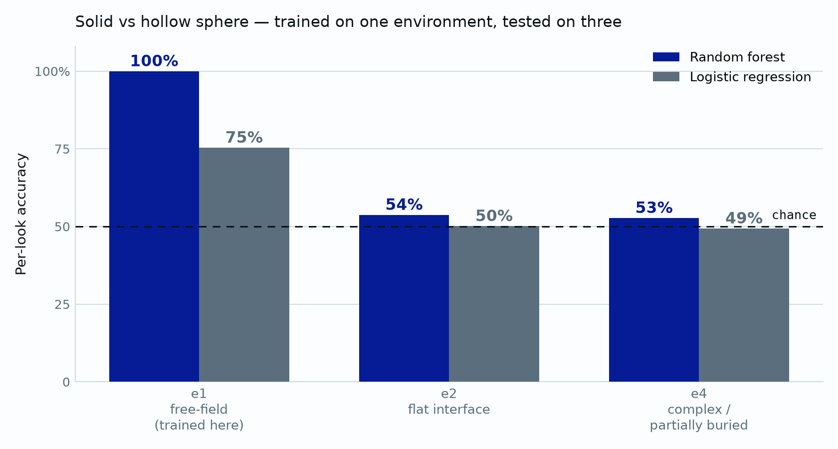
e1. The dashed line is chance for a balanced two-class problem.| Model | e1 · trained | e2 · unseen | e4 · unseen |
|---|---|---|---|
| Random forest | 100.0% | 53.8% | 52.8% |
| Logistic regression | 75.4% | 50.1% | 49.4% |
The random forest separated solid from hollow perfectly inside the environment it was trained in, and was indistinguishable from a coin flip in both environments it had not seen. Logistic regression, with far less capacity to memorise, scored lower in-environment and landed in exactly the same place outside it.
Two mitigations, tested
Multi-look fusion. A single ping is noisy; a real system sees an object many times from many aspects. Averaging class probabilities over K looks of the same run should help. It did not:
| Looks fused | K=1 | K=2 | K=4 | K=8 | K=16 |
|---|---|---|---|---|---|
| Random forest, e2 | 60% | 50% | 50% | 55% | 50% |
| Logistic regression, e2 | 50% | 50% | 50% | 50% | 50% |
No trend. This is the expected outcome once the failure is understood:
averaging suppresses noise, and this is not noise. Every look carries the
same environmental bias, so fusing them reinforces the error rather than
cancelling it. Note also that e2 contains only 20 runs, so these
figures move in 5-point steps: the honest reading is "no effect," not
"a 10-point drop from K=1 to K=2."
An abstention gate. The more useful behavior is refusing to answer. A PCA-space Mahalanobis distance to the training manifold, thresholded at the 90th percentile of training distances, abstains when a look does not resemble anything seen in training. This partly worked:
| Environment | Mean distance | Abstained | Accuracy on accepted (RF) |
|---|---|---|---|
| e2 is a flat interface | 3.34 | 27.9% | 51.6% |
| e4 is complex / buried | 3.76 | 53.8% | 50.8% |
The gate ranked the environments correctly, and without being told anything
about them: it measured e4 as further from training than
e2, and abstained roughly twice as often there. That is the desired
qualitative behavior, and it is worth keeping.
But it did not rescue the decision. Accuracy on the calls it accepted stayed at chance. The gate could tell that the world had changed; it could not find the subset of looks that were still classifiable, because there wasn't one.
Diagnosis
The features were not wrong so much as insufficiently specific. A whitened spectrum and an envelope profile describe the echo as received, and the echo as received is the target's response convolved with everything else in the scene, including the interface, the multipath, the room. In free-field those extra terms are constant, so any consistent difference between the two targets is a valid cue, and a high-capacity model will take whichever cue separates the classes most cleanly. Nothing forces that cue to be the elastic resonance.
Add a reflecting surface and the environmental terms change while the resonance does not. Accuracy collapses to chance, which tells us the model had been leaning almost entirely on the parts that changed.
The 100% is the tell. On real measured data, a perfect score across 400 held-out looks should be read as a warning, not an achievement.
Why this matters beyond a sphere in a lab
Mine countermeasures classifiers are trained on data from one place and deployed in another: different bottom type, different sound-speed profile, different burial state, different vehicle. The in-environment number is the one that is easy to produce and easy to report, and it is the one that means least. Cross-environment evaluation is cheap when a dataset ships an environment ladder, and it is the difference between a result and an artifact.
These features do not support cross-environment classification, and no amount of look-fusion repairs that. The abstention gate is retained: it correctly detects that the environment has changed, which is a genuinely useful property even when it cannot recover the answer.
An earlier version of this test, run on a standard benchmark of pre-extracted band energies with a simulated distribution shift, returned a cautious go. Replacing the simulated shift with a real one reversed the conclusion. That reversal is the most useful thing this exercise produced.
What this does not show
Stated plainly, because these limits are real:
- This is in-air sonar, not underwater. The scattering physics is analogous and the shift is real, but impedance contrasts and scales differ. Nothing here transfers to a Navy problem without being redone in water.
- Spheres are not mines. Canonical targets, controlled facility.
- One training environment. Training across several environments would likely improve generalisation; that is the obvious next experiment, and it is not evidence until it is run.
- The features are deliberately naive. This is a floor, not a ceiling. A physics-informed approach (model-based matched filtering against predicted modal responses, or explicit background subtraction) may well clear the bar these features failed. That is a hypothesis, not a claim.
- Two targets, 60 runs. Small. Sufficient to reject, not to certify.
Next
- Background subtraction before feature extraction, to remove the environmental term the model was leaning on.
- Model-based matched filtering: correlate against predicted modal responses rather than learning free-form features from the raw echo.
- Leave-one-environment-out training across all available environments.
- Re-run in water. Every conclusion here is provisional until then.
Data and reproduction
Blanford, T. (2024). An in-air synthetic aperture sonar dataset of target scattering in environments of varying complexity. figshare. 10.6084/m9.figshare.26961892.v1 · CC BY 4.0. Companion paper: Scientific Data, 10.1038/s41597-024-04050-0.
Transmit: 30→10 kHz linear FM, 500 µs, Tukey 0.1 taper, 100 kHz
sample rate; four receive channels averaged. Features: transmit-whitened log
spectrum 10–30 kHz plus 24-point Hilbert envelope profile, 128-sample window at
the geometrically predicted target range. Models: scikit-learn
LogisticRegression and RandomForestClassifier
(300 trees). Abstention: 8-component PCA, Mahalanobis distance to the training
manifold, threshold at the 90th percentile of training distances.
The harness has not been released. If you want it, ask. Wording and punctuation revised 28 September 2026.
← Mokarran Industries